Looking under the hood of tensorflow models
In this post I will show you how to get more insights into tensorflow models. We’ll cover graph visualization, counting trainable parameters, memory consumption and timing of operations.
Base architecture
All examples in this post use the U-Net1 neural net architecture, which, thanks to many successful applications, gained a lot of attention from the medical image computing community. The network
performs analysis in the left part, where feature maps are downsampled. The right synthesis part of the network upsamples feature maps and concatenates ones coming from corresponding analysis path levels to deliver a fine output in the input resolution.
You can find my implementation of the U-Net model in the blog repository2.
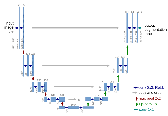 Figure credit: Olaf Ronneberger et al.1
Trainable parameter count
Model complexity relates to the trainable parameter count. You can query the trainable parameter count using the following function:
import tensorflow as tf
import numpy as np

def parameter_count(graph):
  vars = graph.get_collection(tf.GraphKeys.TRAINABLE_VARIABLES)
  return (np.sum([np.prod(v.shape) for v in vars])).value
>>> from u_net import UNet
>>> u_net = UNet()
>>> parameter_count(tf.get_default_graph())
31030658
Peak memory consumption
Peak memory consumption of a model is the factor determining, whether a model will fit on a GPU. A helper function mem_util.peak_memory from the OpenAI repository3 can be used to check the model’s memory consumption. I equipped the UNet class with train and inference methods accepting RunOptions and RunMetadata, which collect debug/profiling information from a session.run() call. The following function returns a dict containing a per device peak memory consumption in bytes:
import tensorflow as tf
import numpy as np
from u_net import UNet
from gradientcheckpointing.test import mem_util # from OpenAI repo

def peak_memory(model, batch_size=1, mode='train'):
  sess = tf.Session()
  sess.run(tf.global_variables_initializer())
  input_shape = [batch_size] + UNet.INPUT_SHAPE
  output_shape = [batch_size] + UNet.OUTPUT_SHAPE
  input_batch = np.random.rand(*input_shape)
  output_batch = np.random.rand(*output_shape)
  run_metadata = tf.RunMetadata()
  options = tf.RunOptions(trace_level=tf.RunOptions.FULL_TRACE)
  if mode == 'train':
    model.train(sess, input_batch, output_batch, options, run_metadata)
  elif mode == 'inference':
    model.inference(sess, input_batch, options, run_metadata)
  return mem_util.peak_memory(run_metadata)
>>> peak_memory(UNet(), mode='train')
{'/cpu:0': 2093226660}
>>> peak_memory(UNet(), mode='inference')
{'/cpu:0': 180936736}
From the above we can see, that the U-Net model requires 180 MB in the inference and ca. 2 GB in the train mode due to the gradient computation.
We can use the peak_memory function to plot train peak memory vs. batch size.
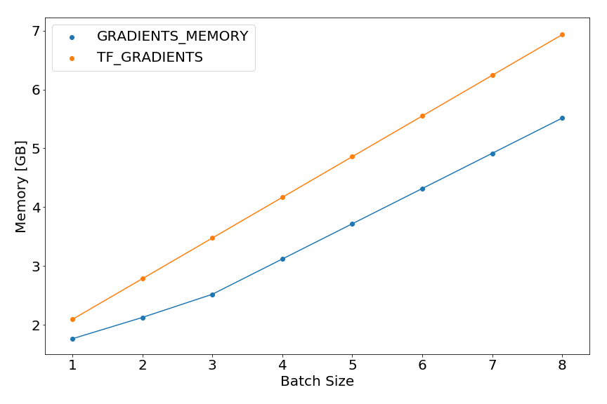 The memory increases linearly with bigger batch size, when we use the standard tensorflow method for gradient computation
 tf.gradients():
optimizer = tf.train.AdamOptimizer()
grads = tf.gradients(self._loss_op, tf.trainable_variables(), gate_gradients=True)
self._train_op = optimizer.apply_gradients(grads_and_vars=list(zip(grads, tf.trainable_variables())))
A similar, but requiring less memory, behavior can be observed for a memory saving gradient computation method published by OpenAI3.
optimizer = tf.train.AdamOptimizer()
grads = gradients_memory(self._loss_op, tf.trainable_variables(), gate_gradients=True)
self._train_op = optimizer.apply_gradients(grads_and_vars=list(zip(grads, tf.trainable_variables())))
For example, for batch size of 8, the peak memory usage can be reduced by 20% with the memory saving gradients.
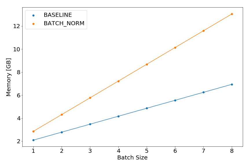
Peak memory analysis can also be used for understanding how the model memory footprint changes with architectural modifications. For instance, let’s plot the train memory footprint of a network with and without batch normalization4 before each nonlinearity.
Timeline
In order to get more information about the running time of graph operations we can use the tf.profiler.profile function.
The code snippet below writes a timeline file:
import tensorflow as tf
import numpy as np
from u_net import UNet

def timeline(model, filename, mode='train'):
  sess = tf.Session()
  sess.run(tf.global_variables_initializer())
  input_shape = [1] + UNet.INPUT_SHAPE
  output_shape = [1] + UNet.OUTPUT_SHAPE
  input_batch = np.random.rand(*input_shape)
  output_batch = np.random.rand(*output_shape)
  run_metadata = tf.RunMetadata()
  options = tf.RunOptions(trace_level=tf.RunOptions.FULL_TRACE)
  if mode == 'train':
    model.train(sess, input_batch, output_batch, options, run_metadata)
  elif mode == 'inference':
    model.inference(sess, input_batch, options, run_metadata)
  builder = (tf.profiler.ProfileOptionBuilder()
    .with_max_depth(6)
    .select(['micros', 'bytes', 'params', 'float_ops'])
    .order_by('peak_bytes'))
  builder = builder.with_timeline_output(filename)
  options = builder.build()
  return tf.profiler.profile(tf.get_default_graph(), run_meta=run_metadata, cmd="scope",
                             options=options)
>>> timeline(UNet(), 'timeline_train.json', mode='train')
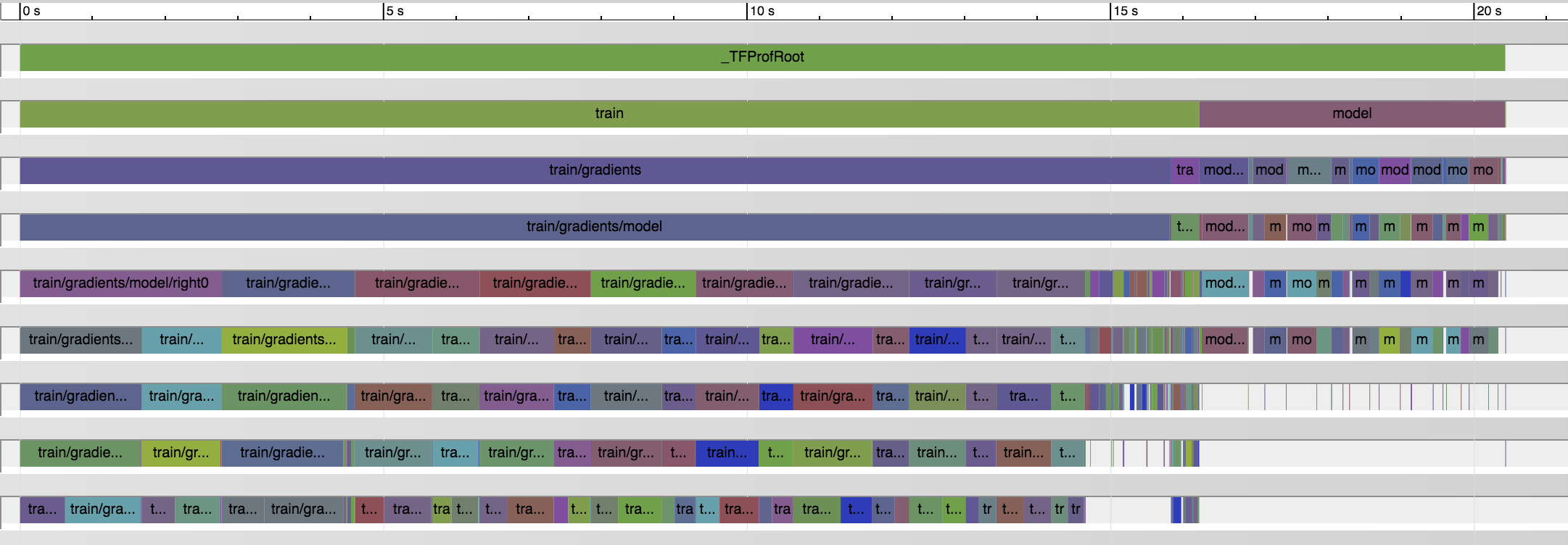
The saved timeline can be opened with a Chrome browser under URL chrome://tracing. From the timeline we can learn about the operation execution order
and how long each operation takes. In the U-Net case (running on a CPU), train ops take around 16 s in comparison to only 5 s required by inference ops.
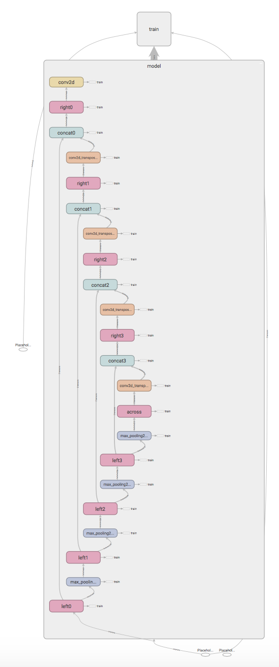
Graph visualization
I find it useful to take a look at my model using TensorBoard to see whether any bugs sneaked in.
The graph definition can be written using the tf.summary.FileWriter class and then displayed using TensorBoard.
I recommend using tf.variable_scope for better graph readability.
# In UNet class definition.
def write_graph(self, filepath):
    writer = tf.summary.FileWriter(filepath, tf.get_default_graph())
>>> model = UNet()
>>> model.write_graph('./graph')
> tensorboard -logdir graph
References
-
Ronneberger et al., U-Net: Convolutional Networks for Biomedical Image Segmentation. MICCAI, 2015. ↩ ↩2
-
Ioffe et al., Batch Normalization: Accelerating Deep Network Training by Reducing Internal Covariate Shift. 2015. ↩