Loss functions for semantic segmentation
Introduction
Categorical cross entropy CCE and Dice index DICE are popular loss functions for training of neural networks for semantic segmentation. In medical field images being analyzed consist mainly of background pixels with a few pixels belonging to objects of interest. Such cases of high class imbalance cause networks to be biased towards background when trained with CCE. To account for that, weighting of foreground and background pixels can be applied. In contrast to CCE, usage of DICE doesn’t require weighting to successfully train models with imbalanced datasets1.
Loss functions
Notation: In the following, \(y_i^j\) and \(\hat{y}_i^j\) denote \(i\)th channel at the \(j\)th pixel location of the reference labels and neural network softmax output, respectively.
\(y^j\) is a one-hot vector of length \(c\) with \(1\) at the reference class location and \(0\) elsewhere.
I use \(c\) to denote the total channel count, \(N\) to denote total pixel count in a mini-batch and \(\epsilon\) as a small constant plugged to avoid numerical problems.
The code examples below use tensorflow and assume that models are fed with 4-D tensors of shape (batch_dim, y_dim, x_dim, channel_dim).
Softmax output: The loss functions are computed on the softmax output which interprets the model output as unnormalized log probabilities and squashes them into \([0,1]\) range such that for a given pixel location \(\sum_{i=0}^c \hat{y}_i = 1\).
Categorical Cross Entropy
Categorical cross entropy sums negative logs of output probabilities for the correct class. Formally, it is defined as:
\[\textrm{cce} = -\sum_i^c \sum_j^N y_i^j\log{\hat{y}_i^j}\]def cce_loss(softmax_output, labels):
eps = 1e-7
log_p = -tf.log(tf.clip_by_value(softmax_output, eps, 1-eps))
loss = tf.reduce_sum(labels * log_p, axis=-1)
return tf.reduce_mean(loss)
Dice
The Dice loss function DICE can be defined as:
\[\textrm{dice\_loss} = 1 - \frac{1}{c}\sum_{i=0}^{c}\frac{\sum_j^N 2y_i^j\hat{y}_i^j + \epsilon}{\sum_j^Ny_i^j + \sum_j^N\hat{y}_i^j + \epsilon}\]or using squares in the denominator (DICE_SQUARE) as proposed by Milletari1:
\[\textrm{dice\_loss\_square} = 1 - \frac{1}{c}\sum_{i=0}^{c}\frac{\sum_j^N 2y_i^j\hat{y}_i^j + \epsilon}{\sum_j^N y_i^jy_i^j + \sum_j^N\hat{y}_i^j\hat{y}_i^j + \epsilon}\]\(\epsilon\) is used to avoid division by 0 (denominator) and to learn from patches containing no pixels of \(i\)th class in the reference (nominator). The multiplication by \(\frac{1}{c}\) gives a nice property, that the loss is within \([0, 1]\) regardless of the channel count. Optionally, the dice loss can be computed only for foreground channels (DICEFG, DICEFG_SQUARE), because it punishes false positives.
def dice_loss(softmax_output, labels, ignore_background=False, square=False):
    if ignore_background:
      labels = labels[..., 1:]
      softmax_output = softmax_output[..., 1:]
    axis = (0,1,2)
    eps = 1e-7
    nom = (2 * tf.reduce_sum(labels * softmax_output, axis=axis) + eps)
    if square:
      labels = tf.square(labels)
      softmax_output = tf.square(softmax_output)
    denom = tf.reduce_sum(labels, axis=axis) + tf.reduce_sum(softmax_output, axis=axis) + eps
    return 1 - tf.reduce_mean(nom / denom)
Experiments
I prepared a toy segmentation task with one foreground class. I used np.random.rand to generate input images.
A pixel is foreground if its value is bigger than some threshold \(\theta\). By tinkering with \(\theta\) we can set the balance between output classes:
- \(\theta\) = 0.95: 95% bg, 5% fg
- \(\theta\) = 0.5: 50% bg, 50% fg
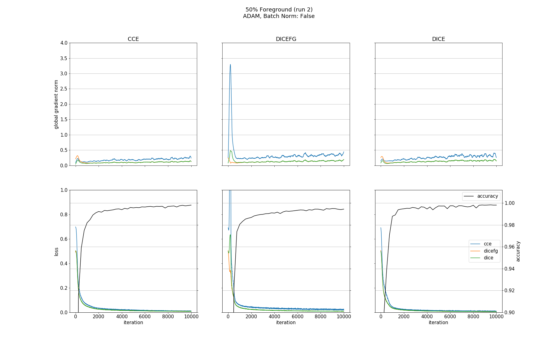
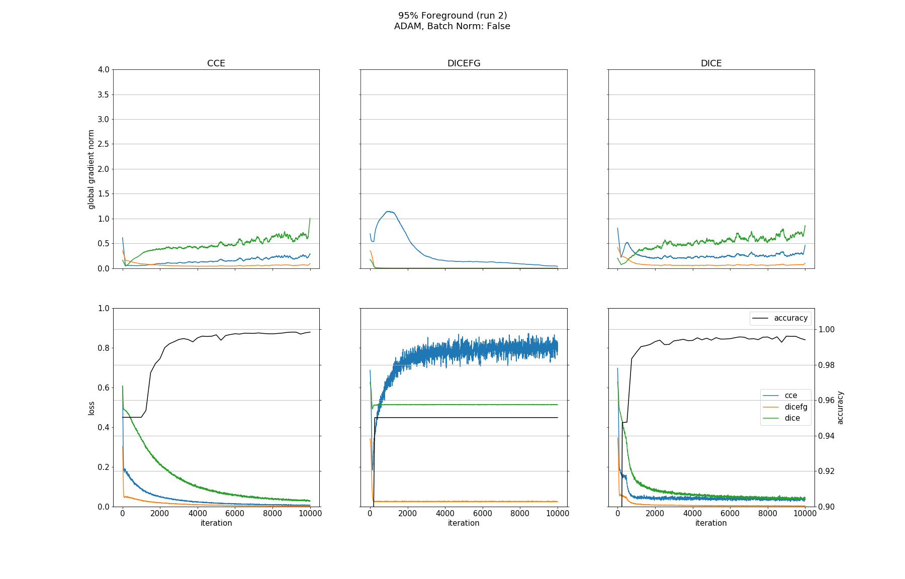
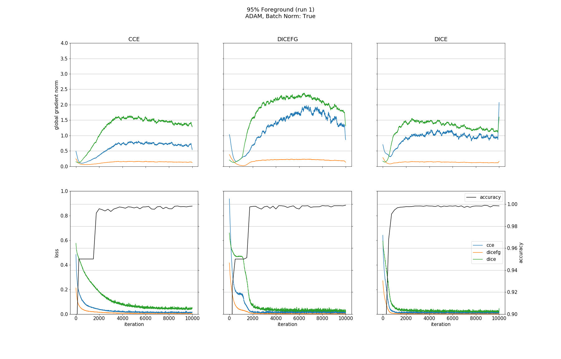
To investigate the behavior of different loss functions I trained a model with one of them for various bg/fg ratios and saved loss values and global gradient norms of all of them. I also trained models with and without batch normalization (BN) before each nonlinearity and used ADAM and SGD optimizers.
You can find my code used for the experiments here2. Feel free to take a look at it and I encourage you to run further experiments using the ipython notebook. Some results are plotted below (column name denotes the loss function used for training). All plots can be found here3.
Results
Please zoom in for better readability.
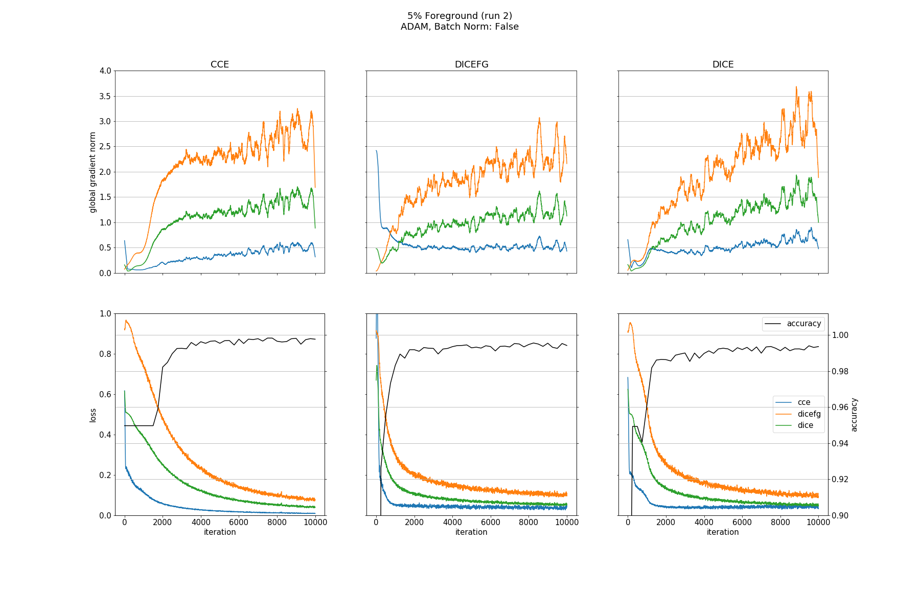
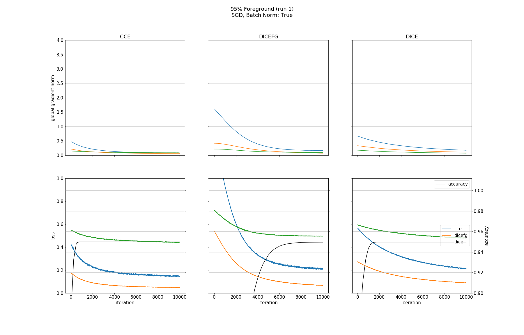
Observations
None of the models converged when optimized with SGD, whether BN was used or not. Optimizing with ADAM made all models without BN converge except for the one trained with DICEFG on the 95% fg data. Using BN before each activation improved models accuracy and helped to train the model with DICEFG on the 95% fg data successfully. When training with DICEFG, the CCE loss and gradient norm skyrocketed in the beginning for the 50% fg dataset.
It is interesting to note, that the gradient norms for the 95% fg case are smaller than those for the 5% fg case. It is a strange observation, because, for example from the point of view of the DICE and CCE loss functions, both situations should be indistinguishable, since they take bg and fg equally into account.
Conclusions
For this toy segmentation task, all models with batch normalization achieved a good accuracy on all bg/fg configurations regardless of the used loss function. Batch normalization improved models performance and was essential to make the model trained with DICEFG converge on the 95% fg dataset.