On Evaluation of Tumor Segmentation
The problem of automatic tumor segmentation is a problem which occupies a lot of researches in the medical imaging field. Having a reliable, automatic segmentation tool would allow for a better and more accurate diagnosis, therapy planing and therapy response assessment. Currently, the standard way to measure the therapy response is to compare the largest diameters of tumors, which clearly neglects the volume change and texture features. With the recent advancements in the field of machine learning, it is only a matter of time before clinicians would have good automatic segmentation tools at their disposal.
Problem
Given reference tumor segmentation produced by a clinical expert and test segmentation output produced by some algorithm for a group of patients, we would like to measure how good the test segmentation is. A patient can have zero or more tumors segmented in the reference. The evaluation should consider two points:
- Detection: How good is my method at finding the tumors?
- Segmentation: How well the tumors my method found are segmented?
Use cases
The evalation criteria should be chosen having the appliaction of an algorithm in mind. We can think of the following scenarios:
- Tumor detection: Were all tumors found? How many false positives per image are produced?
- Tumor volumetry: How accurate is the volume of all found tumors? Tumor volumetry is needed for example for planing of selective internal radiation therapy SIRT, where the activite to be applied depends on the total tumor volume.
- Therapy response classification: Is there a new tumor in the follow-up scan? How has the diameter of target tumors changed since the previous scan?
Definitions
Detection
Detection measures are typically functions of real positives \(P\) (the number of positives in the reference data), real negatives \(N\), true positives \(TP\) (the number of correctly found real positives), true negatives \(TN\), false negatives \(FN\) (the number of missclassified real negatives) and false positives \(FP\). Some of the most common measures are Sensitivity, Specificity, Precision and Recall1:
\[\textrm{Recall} = \textrm{Sensitivity} = \frac{TP}{P}\] \[\textrm{Specificity} = \frac{TN}{N}\] \[\textrm{Precision} = \frac{TP}{TP + FP}\]Precision answers How many relevant items were selected? Recall answers How many selected items are relevant?
Relative volume error
Relative volume error \(\textrm{RVE}\) for a test volume \(A\) and reference volume \(B\) is defined as:
\[\textrm{RVE} = \frac{||A|-|B|}{|B|} \cdot 100\]Jaccard index
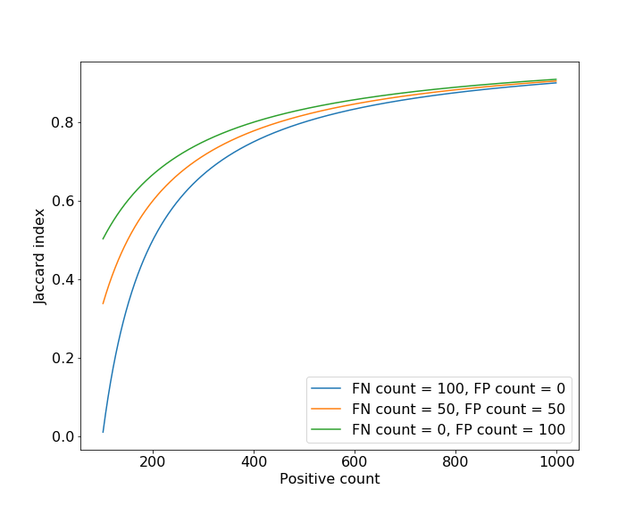
The Jaccard index2 (aka Intersection over Union IoU) is a common metric for evaluation of segmentation quality.
\[0 \leq J(A, B) = \frac{|A \cap B|}{|A \cup B|} = \frac{TP}{TP + FP + FN}\leq 1\]For empty \(A\) and \(B\) the \(J(A,B)=1\). The Jaccard index can be considered a metric, since it satisfies the triangle inequality. Assuming a constant error in terms of missclassified voxels and a variable size of the object to be segmented, the behavior of the Jaccard index as depicted in the following figure can be observed. Note, that Jaccard index yields higher scores for the \(FP=100\) case than for the \(FN=100\).
Dice index or F-1 score
The Dice index3 (aka Dice’s coefficient) is a metric defined very similarly to the Jaccard index, but it does not satisfy the triangle inequality.
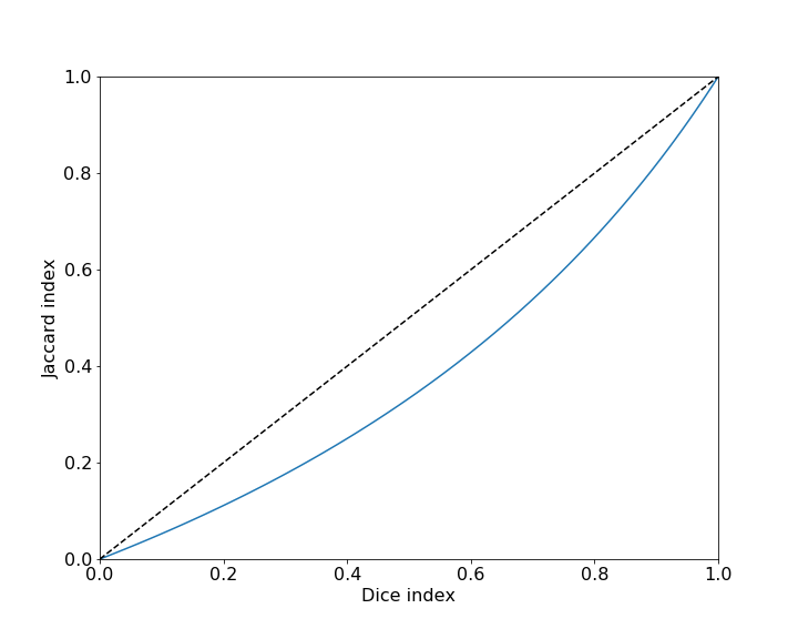
\[0 \leq DSC(A,B) = \frac{2|A \cap B|}{|A|+|B|} = \frac{2J(A,B)}{1+J(A,B)} = \frac{2TP}{2TP + FP + FN} \leq 1\]Dice and Jaccard indices can be in most situations used interchangeably, since Jaccard can be derived from Dice and vice versa. They exhibit the following relationship:
Tversky index
The Tversky index4 is a generalization of the Dice and Jaccard index, where one can weight how the \(FP\) and \(FN\) are weighted. Assuming that \(A\) is a subject of comparison and \(B\) is the referent we can write:
\[S(A,B,\alpha, \beta)_{\alpha, \beta \geq 0} = \frac{|A \cap B|}{|A \cap B| + \alpha|A-B| + \beta|B-A|} = \frac{TP}{TP + \alpha FP + \beta FN}\]By tinkering with \(\alpha\) and \(\beta\) the focus of the comparison can be shifted. In case of \(\alpha > \beta\), the subject features are weighted more heavily than the referent features.
Free-Response Receiver Operating Characteristic (FROC)
FROC5 is an extension to the conventional ROC6 which tries to overcome the limitiation of the ROC which is only one decision per case and only two decision alternatives. The FROC allows for analysis of experiments where number of lesions per case may be zero or more and the reader is allowed to take multiple decisions per image. A typical FROC plot would have Sensitivity on the y-axis and FP per image on the x-axis. It should be noted, that there are currently no established methods to test for significance of differences between two FROC curves as well as no single index summarizing the FROC plot (e.g, ROC has the area under the curve index).
References
-
Tversky A., Features of Similarity. Psychological Review, 1977. ↩
-
Extensions to Conventional ROC Methodology: LROC, FROC, and AFROC. Journal of the International Commission on Radiation Units and Measurements, 2008. ↩