LRP for semantic segmentation
Layer-wise relevance propagation
Layer-wise relevance propagation allows to obtain a pixel-wise decomposition of a~model decision and is applicable for most state-of-the-art architectures for image classification and neural reinforcement learning1. LRP uses a notion of relevance \(R\) which is equal to the model output for the output neurons and can be propagated to lower layers.
LRP for image classification
LRP can be employed to explain classification decisions for a given class \(i\) by relevance propagation from the corresponding model output $y^i$ according to:
\[y^i = R = \ldots = \sum_{d \in L^l} R_d^{(l)} = \ldots = \sum_{d \in L^1} R_d^{(1)} = \sum M^i \ldots (1)\]where \(l\) refers to the layer index, \(L^l\) to all neurons of layer \(l\), and \(R_d^{(l)}\) to a relevance of neuron \(d\) in layer \(l\). Typically, the relevances are propagated to the input layer (\(l=1\)) yielding a relevance map \(M^i\), which enables visualization of input regions influencing the model decision.
LRP for semantic segmentation
In order to apply LRP to semantic segmentation models, we cast the segmentation problem as a voxel-wise classification. This means that in order to explain a decision of a segmentation model for a given output region \(A\), we propose to compute the input relevance maps according to Eq.1 for each considered output location \(a \in A\). Then the relevance map \(M^i\) explaining the model decision for class \(i\) in the region \(A\) can be calculated as:
\[M^i_A = \sum_{a \in A} \frac{M_a^i}{\sum M_a^i}\]We normalize \(M_a^i\) by its sum to ensure that each output location \(a\) equally contributes to the final relevance map \(M^i\).
Relevance analysis of liver tumor segmentation CNN
We train a 3D u-net2 with a 6-channel input and 2-channel output to segment liver tumors in : T2, non contrast enhanced T1 (plain-T1), and four dynamic contrast enhanced (DCE) T1 images acquired 20s (T1-20s), 60s (T1-60s), 120s (T1-120s), and 15min (T1-15min) after contrast agent administration (Gd-EOB-DTPA). All sequences were motion corrected using the T1-15min image as reference3.
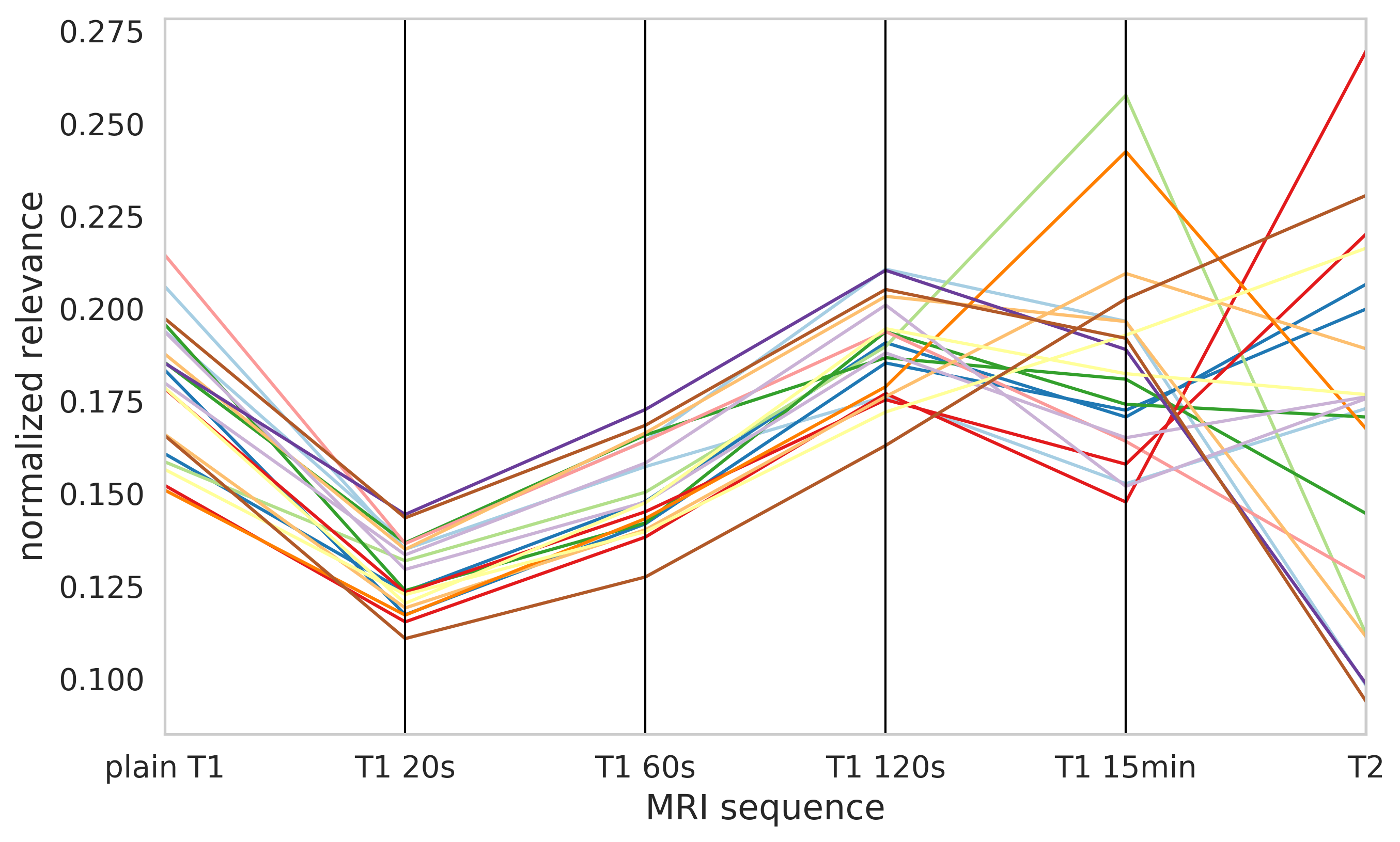
MRI sequence relevance
Normalized relevance distribution across input MRI sequences for 20 test patients denoted by different colors.
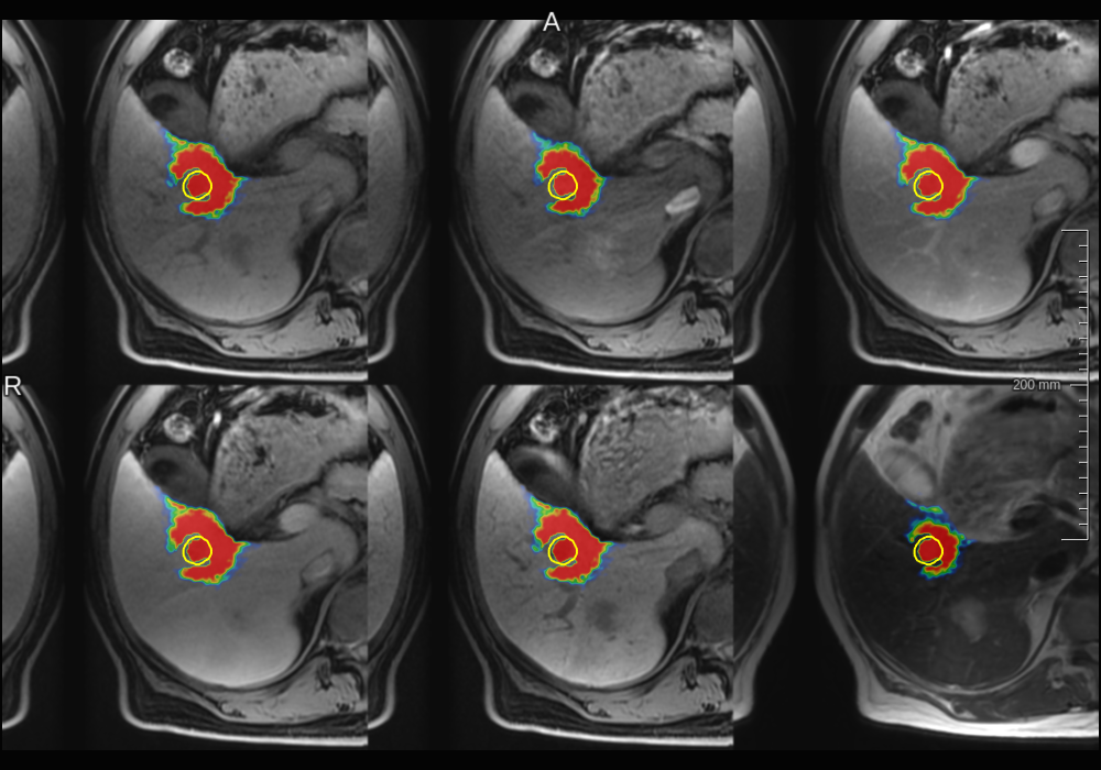
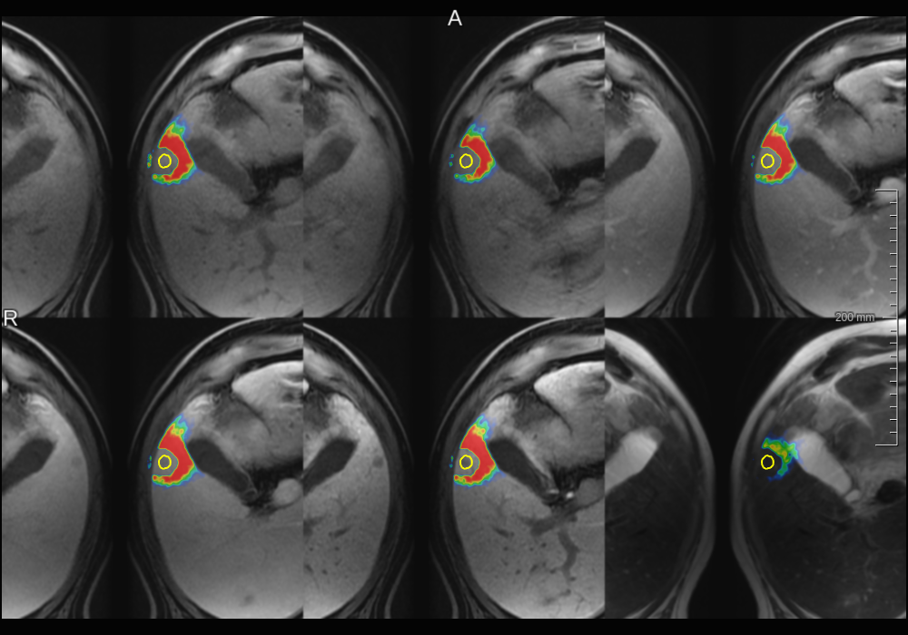
Pixel-level explanations
Foreground relevance maps computed for a true positive.
Foreground relevance maps computed for a false negative.
Discussion
- CNN used information from all MRI sequences.
- T1-15min sequence, which was used to create training labels was not the most important one.
- Similar relevance attribution for plain T1, T1-20s, T1-60s, and T1-120s.
- Pixel-level explanations are hard to interpret.
References
-
S. Bach et al., On pixel-wise explanations for non-linear classifier decisions by layer-wise relevance propagation. PLOS ONE, 2015. ↩
-
Ö. Çiçek et al. 3d u-net: learning dense volumetric segmentation from sparse annotation. MICCAI, 2016. ↩
-
J. Strehlow et al. Landmark-based evaluation of a deformable motion correction for dce-mri of the liver. IJCARS, 2018. ↩